- GloWPa
- 1 Installation
- 2 Model Input
- 3 Model Setup
- 4 Run GloWPa
- 5 Model Output
- 6 Contributing
- Datasets
- References
GloWPa
The GloWPa (Global Waterborne Pathogen) model simulates emissions of pathogens (currently Cryptosporidium and Rotavirus) to surface water (Hofstra & Vermeulen, 2016). These pathogens are known to be a leading cause of diarrhoeal diseases among people that are exposed to high concentrations. GloWPa focuses on human and livestock emissions of pathogens that end up in surface water systems through various pathways.
1 Installation
The GloWPa model R package can be installed from the GitLab repository
using the R package devtools. Install the master version from
GitLab:
install.packages("devtools")
devtools::install_gitlab("glowpa/glowpa-r",host="https://git.wur.nl/")
You can also install other versions from GitLab by extending the
repository address using the format username/repo[@ref]. To install
tagged versions like e.g. 0.1.0 version you can use:
devtools::install_gitlab("glowpa/glowpa-r@0.1.0",host="https://git.wur.nl/")
Run example:
library(glowpa)
example("glowpa_start", echo = FALSE)
#> Warning in file(con, "r"): file("") only supports open = "w+" and open = "w+b":
#> using the former
2 Model Input
A set of data sources has been collected and is available on request.
The prepare_data function can be used to generate global or country
scale model input at a given GADM level and various spatial resolutions
based on this pre-defined set of data sources. More information about
the data sources can be found in section Datasets
library(glowpa)
datasource_dir <- "/home/data/glowpa/datasources"
# generate global input data at 30min (0.5 deg) resolution using country borders
prepare_data(datasource_dir, "input/global", res = 0.5, country = NA, level = 0)
# generate Uganda input data at 5min resolution using GADM level 1 borders.
prepare_data(datasource_dir, "input/uga"  , res = 5/60, country = "UGA", level = 1)
3 Model Setup
The model setup needs to specified in a yaml configuration file.
3.1 Model Options
population:
  correct: TRUE # TRUE | FALSE
wwtp:
  treatment: AREA # AREA | POINT
livestock:
  enabled: FALSE # TRUE | FALSE
hydrology:
  enabled: FALSE # TRUE | FALSE
pathogen: rotavirus # rotavirus | cryptosporidium | any other
| keys | description | default |
|---|---|---|
| population.correct | Option to correct the gridded population data to match the total population as specified in the human isodata file. It is usefull to turn off this option in case you want to run mutiple or a single basins(s) and your domain includes partitial countries. | TRUE |
| wwtp.treatment | Option to control the waste waster treatment locations. The model includes a waste water treatment plant in each grid cell when the option is set to AREA. The option POINT must be used in case the locations of waste water treatment pants are known. | AREA |
| livestock.enabled | Option to enable/disable the livestock module. When TRUE the model will include pathogen emissions from livestock animals. Please read section Livestock Input |
FALSE |
| hydrology.enabled | Option to enable/disable the hydrology module. When TRUE the model will use the river network to route the pathogen emissions to water. Please read section Hydrology Input |
FALSE |
| pathogen | Option controlling the selected pathogen (and related properties) for the model simulation. The selected pathogen name must be available in the internal model defaults or pathogen input file. | rotavirus |
3.2 Logger Settings
logger:
  enabled: TRUE # TRUE | FALSE
  threshold: <value>    # FATAL | ERROR | WARN | SUCCESS | INFO | DEBUG | TRACE
  file: <path_to_file>
  appender: CONSOLE # CONSOLE | FILE | TEE
| keys | description | required | default | values |
|---|---|---|---|---|
| enabled | option to set logging ON | OFF | no | TRUE | TRUE / FALSE |
| threhold | log level threshold | no | INFO | OFF | FATAL | ERROR | WARN | SUCCESS | INFO | DEBUG | TRACE |
| file | path to log file | yes | no | e.g. ouput/glowpa.log | |
| appender | log destination | no | CONSOLE | CONSOLE | FILE (file only) | TEE (file + console |
3.3 Input Settings
3.3.1 Human Input
input:
  isoraster: <path_to_file>
  isodata: <path_to_file>
  wwtp: <path_to_file>
  pathogen: <path_to_file>
  population:
    urban: <path_to_file>
    rural: <path_to_file>
| keys | description | data_format |
|---|---|---|
| isoraster | The isoraster input file assigns administrative areas in the gridded domain. Besides in determines the model domain and resolution. | tif |
| isodata | The isodata file holds all data of the administrative areas. | RDS |
| wwtp | The wwtp input file holds information about the waste water treatment plants in the modelling domain. By default the model assumes a waste water treatment plant in each administrative area. | RDS |
| pathogen | The pathogen input file holds the properties of a chosen set of pathogens | RDS |
| population.urban | Raster file holding the urban population. | tif |
| population.rural | Raster file holding the rural population. | tif |
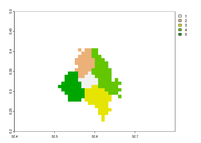
Isoraster
The isoraster input file is used to produce gridded output of pathogen emissions by mapping the isodata properties by iso to the model grid cells. The isoraster also determines the model resolution, domain and mask. All no data values will be masked. Example of isoraster grid:
isoraster_file <- system.file("extdata/kla/isoraster_kla.tif", package = "glowpa")
isoraster <- terra::rast(isoraster_file)
terra::plot(isoraster)
Isodata
Example of the isodata file:
isodata_file <- system.file("extdata/kla/glowpa_isodata_kla.RDS", package = "glowpa")
df_isodata <- readRDS(isodata_file)
head(df_isodata)
| iso | gid | iso_country | subarea | hdi | population | fraction_urban_pop | fraction_pop_under5 | sheddingRate_virus | shedding_duration_virus | incidence_urban_under5_virus | incidence_urban_5plus_virus | incidence_rural_under5_virus | incidence_rural_5plus_virus | sheddingRate_protozoa | shedding_duration_protozoa | incidence_urban_under5_protozoa | incidence_urban_5plus_protozoa | incidence_rural_under5_protozoa | incidence_rural_5plus_protozoa | flushSewer_urb | flushSeptic_urb | flushPit_urb | flushOpen_urb | flushUnknown_urb | pitSlab_urb | pitNoSlab_urb | compostingToilet_urb | bucketLatrine_urb | containerBased_urb | hangingToilet_urb | openDefecation_urb | other_urb | coverBury_urb | sewageTreated_urb | fecalSludgeTreated_urb | isWatertight_urb | hasLeach_urb | emptyFrequency_urb | pitAdditive_urb | urine_urb | twinPits_urb | onsiteDumpedland_urb | flushSewer_rur | flushSeptic_rur | flushPit_rur | flushOpen_rur | flushUnknown_rur | pitSlab_rur | pitNoSlab_rur | compostingToilet_rur | bucketLatrine_rur | containerBased_rur | hangingToilet_rur | openDefecation_rur | other_rur | coverBury_rur | sewageTreated_rur | fecalSludgeTreated_rur | isWatertight_rur | hasLeach_rur | emptyFrequency_rur | pitAdditive_rur | urine_rur | twinPits_rur | onsiteDumpedland_rur | fEmitted_inEffluent_after_treatment_virus | fEmitted_inEffluent_after_treatment_protozoa |
|---|---|---|---|---|---|---|---|---|---|---|---|---|---|---|---|---|---|---|---|---|---|---|---|---|---|---|---|---|---|---|---|---|---|---|---|---|---|---|---|---|---|---|---|---|---|---|---|---|---|---|---|---|---|---|---|---|---|---|---|---|---|---|---|---|---|---|---|
| 1 | UGA.16.1.1_1 | UGA | Central Division | 0.493 | 63206 | 1 | 0.1772789 | 1e+10 | 7 | 0.24 | 0.08 | 0.24 | 0.08 | 1e+09 | 7 | 0.24 | 0.08 | 0.24 | 0.08 | 0.2634261 | 0.2023951 | 0.0572373 | 0.0122217 | 0.0077538 | 0.4109741 | 0.0244770 | 0.0068359 | 0 | 0 | 0.0000000 | 0.0115781 | 0.0031009 | 0 | 1 | 0.4367804 | 0 | 0.7334575 | 3 | 0 | 0.0068359 | 0.1 | 0.1 | 0.2634261 | 0.2023951 | 0.0572373 | 0.0122217 | 0.0077538 | 0.4109741 | 0.0244770 | 0.0068359 | 0 | 0 | 0.0000000 | 0.0115781 | 0.0031009 | 0 | 1 | 0.4367804 | 0 | 0.7334575 | 3 | 0 | 0.0068359 | 0 | 0 | 0.5 | 0.25 |
| 2 | UGA.16.1.2_1 | UGA | Kawempe Division | 0.493 | 333024 | 1 | 0.1772789 | 1e+10 | 7 | 0.24 | 0.08 | 0.24 | 0.08 | 1e+09 | 7 | 0.24 | 0.08 | 0.24 | 0.08 | 0.0368606 | 0.1422745 | 0.0576013 | 0.0016796 | 0.0052485 | 0.7361309 | 0.0144162 | 0.0003307 | 0 | 0 | 0.0001061 | 0.0045987 | 0.0007456 | 0 | 1 | 0.2112449 | 0 | 0.7055242 | 3 | 0 | 0.0003307 | 0.1 | 0.1 | 0.0368606 | 0.1422745 | 0.0576013 | 0.0016796 | 0.0052485 | 0.7361309 | 0.0144162 | 0.0003307 | 0 | 0 | 0.0001061 | 0.0045987 | 0.0007456 | 0 | 1 | 0.2112449 | 0 | 0.7055242 | 3 | 0 | 0.0003307 | 0 | 0 | 0.5 | 0.25 |
| 3 | UGA.16.1.3_1 | UGA | Makindye | 0.493 | 385309 | 1 | 0.1772789 | 1e+10 | 7 | 0.24 | 0.08 | 0.24 | 0.08 | 1e+09 | 7 | 0.24 | 0.08 | 0.24 | 0.08 | 0.0285704 | 0.2592807 | 0.0825400 | 0.0038217 | 0.0174771 | 0.5746897 | 0.0242897 | 0.0014008 | 0 | 0 | 0.0000345 | 0.0060824 | 0.0018341 | 0 | 1 | 0.2364107 | 0 | 0.7400310 | 3 | 0 | 0.0014008 | 0.1 | 0.1 | 0.0285704 | 0.2592807 | 0.0825400 | 0.0038217 | 0.0174771 | 0.5746897 | 0.0242897 | 0.0014008 | 0 | 0 | 0.0000345 | 0.0060824 | 0.0018341 | 0 | 1 | 0.2364107 | 0 | 0.7400310 | 3 | 0 | 0.0014008 | 0 | 0 | 0.5 | 0.25 |
| 4 | UGA.16.1.4_1 | UGA | Nakawa Division | 0.493 | 317023 | 1 | 0.1772789 | 1e+10 | 7 | 0.24 | 0.08 | 0.24 | 0.08 | 1e+09 | 7 | 0.24 | 0.08 | 0.24 | 0.08 | 0.0986067 | 0.2822786 | 0.0659453 | 0.0027247 | 0.0160244 | 0.4979573 | 0.0274612 | 0.0005599 | 0 | 0 | 0.0006785 | 0.0069328 | 0.0008310 | 0 | 1 | 0.1906296 | 0 | 0.7880375 | 3 | 0 | 0.0005599 | 0.1 | 0.1 | 0.0986067 | 0.2822786 | 0.0659453 | 0.0027247 | 0.0160244 | 0.4979573 | 0.0274612 | 0.0005599 | 0 | 0 | 0.0006785 | 0.0069328 | 0.0008310 | 0 | 1 | 0.1906296 | 0 | 0.7880375 | 3 | 0 | 0.0005599 | 0 | 0 | 0.5 | 0.25 |
| 5 | UGA.16.1.5_1 | UGA | Rubaga Division | 0.493 | 383216 | 1 | 0.1772789 | 1e+10 | 7 | 0.24 | 0.08 | 0.24 | 0.08 | 1e+09 | 7 | 0.24 | 0.08 | 0.24 | 0.08 | 0.0046542 | 0.1646388 | 0.0895414 | 0.0017990 | 0.0107916 | 0.6888292 | 0.0310096 | 0.0005665 | 0 | 0 | 0.0000201 | 0.0037351 | 0.0043923 | 0 | 1 | 0.2438574 | 0 | 0.9892711 | 3 | 0 | 0.0005665 | 0.1 | 0.1 | 0.0046542 | 0.1646388 | 0.0895414 | 0.0017990 | 0.0107916 | 0.6888292 | 0.0310096 | 0.0005665 | 0 | 0 | 0.0000201 | 0.0037351 | 0.0043923 | 0 | 1 | 0.2438574 | 0 | 0.9892711 | 3 | 0 | 0.0005665 | 0 | 0 | 0.5 | 0.25 |
The supporting table with column names and descriptions does contain
placeholders for pathogen_type (virus/protozoa) and area_type
(urb/rur) to limit the table length.
| column | description |
|---|---|
| iso | Iso identifier in isoraster input file |
| iso_country | ISO3 Alpha code of country |
| population | Total population in administrative area used as reference for correcting gridded population data. |
| fraction_urban_pop | Fraction of urban population in administrative area for correcting gridded population data |
| fraction_pop_under5 | Fraction population younger than 5 years. |
| sheddingRate_{pathogen_type} | Shedding rate for pathogen_type |
| shedding_duration_{pathogen_type} | Shedding duration for pathogen_type |
| incidence_{area_type}_under5_{pathogen_type} | Incidence rate (new infections/people) for pathogen_type under children (< 5 years) in area_type areas |
| incidence_{area_type}_5plus_{pathogen_type} | Incidence rate (new infections/people) for pathogen_type under children (> 5 years) and adults in area_type areas. |
| flushSewer_{area_type} | Fraction of people connected to flush sewer in area_type areas. |
| flushSeptic_{area_type} | Fraction of people using flush septic tanks in area_type areas. |
| flushPit_{area_type} | Fraction of people using flush pit sanitation in area_type areas. |
| flushOpen_{area_type} | Fraction of people using flush open sanitation in area_type areas |
| flushUnknown_{area_type} | Fraction of people using flush to unknown place in area_type areas. |
| pitSlab_{area_type} | Fraction of people using pits with slab sanitation in area_type areas. |
| pitNoSlab_{area_type} | Fraction of people using open pit sanitation in area_type areas. |
| compostingToilet_{area_type} | Fraction of people using composting toilets in area_type areas. |
| bucketLatrine_{area_type} | Fraction of people using bucket latrines in area_type areas |
| containerBased_{area_type} | Fraction of people using container based sanitation in area_type areas |
| hangingToilet_{area_type} | Fraction of people using hanging toilets/latrines in area_type areas |
| openDefecation_{area_type} | Fraction of people using open defecation sanitation in area_type areas |
| other_{area_type} | Fraction of people using other sanitation type in area_type areas. |
| onsiteDumpedland_{area_type} | fraction of fecal sludge which is dumped on land in area_type areas. |
| coverBury_{area_type} | ? |
| sewageTreated_{area_type} | Fraction the sewerage system which will have waste water treatment in area_type areas. |
| fecalSludgeTreated_{area_type} | Fraction the fecal sludge which will have treatment in area_type areas. |
| isWatertight_{area_type} | ? |
| hasLeach_{area_type} | Fraction of ? |
| emptyFrequency_{area_type} | Empty frequency per year of ? |
| pitAdditive_{area_type} | ? |
| urine_{area_type} | ? |
| twinPits_{area_type} | ? |
| fEmitted_inEffluent_after_treatment_{pathogen_type} | Fraction of pathogens emitted after treatment for pathogen_type |
WWTP
The emissions from sanitation systems connected to waste water treatment plants (WWTP) are distributed over the treatment locations based on the capacity relatively to the total country capacity. This methodology requires at least one WWTP location per country in the modelling domain. If this condition is not met, the model does not treat the waste water and all emissions are directly released to the surface water.
wwtp_file <- system.file("extdata/kla/wwtp_kla.RDS",package = "glowpa")
wwtp <- readRDS(wwtp_file)
head(wwtp)
| lon | lat | subregion | capacity | treatment_type |
|---|---|---|---|---|
| 32.60759 | 0.3184881 | Bugolobi | 33000 | Secondary |
| 32.54433 | 0.3465463 | Kasubi | 5400 | Primary |
| column | description |
|---|---|
| lon | Longitude (decimal degrees) of waste water treatment plant |
| lat | Latitude (decimal degrees) of waste water treatment plant |
| capacity | Amount of people connected to waste water treatment plant |
| treatment_type | Level of treatment. One of Primary, Secondary, Tertiary |
Pathogen
The pathogen input file is tabular data holding properties of various
pathogens selected by the modeler. Currently only the name and
pathogen_type is used to estimate the pathogen loads from human
emissions. The declared pathogen in the model settings is used to lookup
the pathogen properties by name.
Example:
| name | pathogen_type | Tcoeff_1 | Tcoeff_2 | storage_time | storage_time_low | retention_lower | retention_upper | lambda | Kt | kl | kd | v_settling |
|---|---|---|---|---|---|---|---|---|---|---|---|---|
| cryptosporidium | Protozoa | -2.5586000 | 119.6300000 | 274 | 30 | 3.2000000 | 8.80000 | 0.158 | 0.0051 | 0.0004798 | 9.831 | 0.1 |
| rotavirus | Virus | 0.0089028 | 0.0397288 | NA | NA | 0.4569258 | 3.09691 | NA | NA | 0.0000471 | NA | NA |
| column | description | required |
|---|---|---|
| name | Name of the pathogen used as lookup table for the selected pathogen in the model settings. | yes |
| pathogen_type | the type of pathogen used to estimate human emissions from sanitation. Should be one of Virus, Protozoa, Bacteria, Helminth. | yes |
| Tcoeff_1 | The rate constant a in y(x) = ax + b which describes how the T90 survival depends on temperature (x). |
yes, when livestock.enabled is TRUE. Otherwise no. |
| Tcoeff_2 | The interception constant b in y(x) = ax + b which describes how the T90 survival depends on temperature (x). |
yes, when livestock.enabled is TRUE. Otherwise no. |
| storage_time | The manure storage time in days. Used to calculate the survival fraction of the total pathogen load in the manure storage (> 1 month) before spreading to land. | yes, when livestock.enabled is TRUE. Otherwise no. |
| storage_time_low | The manure storage time in days. Used to calculate the survival fraction of the total pathogen load in the manure storage (< 1 month) before spreading to land. Only for pigs there is one storage system for which a shorter storage time is assumed. | yes, when livestock.enabled is TRUE. Otherwise no. |
| retention_lower | The log10 oocyst retention upper boundary condition from vegetated plots under field conditions with surface runoff values ranging from 0-20mm | yes, when hydrology.enabled is TRUE. Otherwise no. |
| retention_upper | The log10 oocyst retention lower boundary condition from vegetated plots under field conditions with surface runoff values ranging from 0-20mm. | yes, when hydrology.enabled is TRUE. Otherwise no. |
| lambda | Dimensionless constant to estimate the temperature related decay coefficient. | yes, when hydrology.enabled is TRUE. Otherwise no. |
| Kt | Temperature related decay rate coefficient (day-1) at 4° C | yes, when hydrology.enabled is TRUE. Otherwise no. |
| kl | Proportionally constant (m^2 kJ-1) to estimate the solar radiation-dependent decay rate coefficient. | yes, when hydrology.enabled is TRUE. Otherwise no. |
| kd | Proportionally constant (L mg-1 m-1) to estimate the attenuation coefficient (m-1) as function from DOC concentrations (mg L-1). | yes, when hydrology.enabled is TRUE. Otherwise no. |
| v_settling | Settling velocity (m day-1). Used to determine the decay rate coefficient related to sedimentation processes in rivers. | yes, when hydrology.enabled is TRUE. Otherwise no. |
3.3.2 Livestock Input
The methodology to calculate pathogen emissions from livestock animals has been described by Vermeulen et al. (2017).
input:
  temperature:
    year: <path_to_file>
  manure:
    management_systems: <path_to_file>
  livestock:
    animal_isoraster: <path_to_file>
    production_systems: <path_to_file>
    manure_fractions: <path_to_file>
    animals:
      asses:
        isodata: <path_to_file>
        heads: <path_to_file>
      buffaloes:
        isodata: <path_to_file>
        heads: <path_to_file>
      camels:
        isodata: <path_to_file>
        heads: <path_to_file>
      cattle:
        isodata: <path_to_file>
        heads: <path_to_file>
      chickens:
        isodata: <path_to_file>
        heads: <path_to_file>
      ducks:
        isodata: <path_to_file>
        heads: <path_to_file>
      goats:
        isodata: <path_to_file>
        heads: <path_to_file>
      horses:
        isodata: <path_to_file>
        heads: <path_to_file>
      mules:
        isodata: <path_to_file>
        heads: <path_to_file>
      pigs:
        isodata: <path_to_file>
        heads: <path_to_file>
      sheep:
        isodata: <path_to_file>
        heads: <path_to_file>
| keys | description | required |
|---|---|---|
| temperature.year | Raster file holding the yearly averaged temperatures in degrees Celsius. | Yes, when livestock.enabled is set to TRUE |
| manure.management_systems | Tabular data holding the fractions of various manure management systems for each livestock type in the administrative areas. | Yes, when livestock.enabled is set to TRUE |
| livestock.animal_isoraster | Isoraster holding the iso values used in any of the specified livestock/animal input files. | No. Only provide different isoraster for livestock when different iso values or areas are used in livestock input data. |
| livestock.production_systems | Table data file holding fractions of intensive and extensive livestock systems for each livestock type and iso area | Yes, when livestock.enabled is set to TRUE. |
| livestock.manure_fractions | Table data file holding fraction of manure either going direct to land or to other uses for each livestock type, production system and iso area. | Yes, when livestock.enabled is set to TRUE |
| livestock.animals.<animal_type>.isodata | Table data file holding properties used to calculate the pathogen emissions from the animal manure for each iso area. | Yes, when livestock.enabled is set to TRUE. A separated isodata input file must be specified for asses, buffaloes, camels, cattle, chickens, ducks, goats, horses, mules, pigs, sheep. |
| livestock.animals.<animal_type>.heads | Raster data holding the number of animals | Yes, when livestock.enabled is set to TRUE. A separated isodata input file must be specified for asses, buffaloes, camels, cattle, chickens, ducks, goats, horses, mules, pigs, sheep. |
Manure Management Systems
The manure management systems input is tabular data holding the fractions of various manure management systems for each livestock type in the administrative areas. The data column can be missing if any of the specified manure management systems is not applicable on a given livestock type. The model will consider this fraction to be zero. The following livestock types must be prepared:
- cattle
- buffaloes
- pigs
- poultry
- sheep
- goats
- horses
- asses
- mules
- camels
According to the description, used for fuel includes both manure going to anaerobic digesters and manure that is burned for fuel. We therefore assume that half of the manure in this category leaves the system, and the other half ends up on land after a 2 log reduction in infectivity.
| column | description | ipcc_2006 | usepa_1992 | storage_time |
|---|---|---|---|---|
| iso | Iso identifier in either isoraster input file or animal isoraster file. | - | - | - |
| PP_* | Fraction manure in pasture/range/paddock. | pasture/range/paddock | pasture/range/paddock | NA |
| DS_* | Fraction manure daily spread on land. | daily spread | daily spread | 0 days |
| SS_* | Fraction solid storage. | solid storage | solid storage & dry lot | long storage |
| DL_* | Fraction dry lot storage. | dry lot | - | long storage |
| LS_* | Fraction liquid/slurry storage. | lidquid/slurry | liquid systems (includes liquid/slurry storage and pit storage) | long storage |
| UAL_* | Fraction uncovered anaerobic lagoon. | lagoon | anaerobic lagoon | long storage |
| AD_* | Fraction anaerobic digester. | anaerobic digester | - | NA |
| BF_* | Fraction burned for fuel. | burned for fuel | used for fuel | NA |
| Pl1_* | Fraction pit storage shorter than 1 month. | pit < 1 month | - | short storage |
| Ph1_* | Fraction pit storage longer than 1 month. | pit > 1 month | - | long storage |
| SSDL_* | Fraction solid storage & dry lot | - | solid storage & dry lot | long storage |
| O_* | Fraction other systems. | other | other (includes deep pit stacks, litter, and other) | long storage |
example:
| iso | country | CC | PP_dairy | DS_dairy | SS_dairy | DL_dairy | LS_dairy | UAL_dairy | AD_dairy | BF_dairy | O_dairy | PP_meat | DS_meat | SS_meat | DL_meat | LS_meat | UAL_meat | AD_meat | BF_meat | O_meat | PP_cattle | DS_cattle | SS_cattle | DL_cattle | LS_cattle | UAL_cattle | AD_cattle | BF_cattle | O_cattle | Tot_cattle | Tot2_cattle | PP_buffaloes | DS_buffaloes | SS_buffaloes | DL_buffaloes | LS_buffaloes | UAL_buffaloes | AD_buffaloes | BF_buffaloes | O_buffaloes | Tot_buffaloes | Tot2_buffaloes | UAL_pigs | LS_pigs | SS_pigs | DL_pigs | Pl1_pigs | Ph1_pigs | DS_pigs | AD_pigs | O_pigs | Tot_pigs | Tot2_pigs | UAL_poultry | LS_poultry | DS_poultry | SSDL_poultry | PP_poultry | BF_poultry | O_poultry | Tot_poultry | UAL_sheep | LS_sheep | DS_sheep | SSDL_sheep | PP_sheep | BF_sheep | O_sheep | Tot_sheep | UAL_goats | LS_goats | DS_goats | SSDL_goats | PP_goats | BF_goats | O_goats | Tot_goats | UAL_horses | LS_horses | DS_horses | SSDL_horses | PP_horses | BF_horses | O_horses | Tot_horses | UAL_mules | LS_mules | DS_mules | SSDL_mules | PP_mules | BF_mules | O_mules | Tot_mules | UAL_asses | LS_asses | DS_asses | SSDL_asses | PP_asses | BF_asses | O_asses | Tot_asses | UAL_camels | LS_camels | DS_camels | SSDL_camels | PP_camels | BF_camels | O_camels | Tot_camels |
|---|---|---|---|---|---|---|---|---|---|---|---|---|---|---|---|---|---|---|---|---|---|---|---|---|---|---|---|---|---|---|---|---|---|---|---|---|---|---|---|---|---|---|---|---|---|---|---|---|---|---|---|---|---|---|---|---|---|---|---|---|---|---|---|---|---|---|---|---|---|---|---|---|---|---|---|---|---|---|---|---|---|---|---|---|---|---|---|---|---|---|---|---|---|---|---|---|---|---|---|---|---|---|---|---|---|---|---|---|---|
| 4 | Afghanistan | ME | 0.80 | 0.020 | 0.02 | 0 | 0.010 | 0.00 | 0.00 | 0.17 | 0.00 | 0.79 | 0.02 | 0 | 0.01 | 0 | 0 | 0 | 0.17 | 0.02 | 0.795 | 0.020 | 0.010 | 0.005 | 0.005 | 0.00 | 0.00 | 0.170 | 0.01 | 1.015 | 0.045 | 0.20 | 0.19 | 0 | 0.00 | 0.00 | 0 | 0 | 0.42 | 0.19 | 1 | 0.38 | 0.00 | 0.14 | 0.00 | 0.69 | 0.000 | 0.170 | 0.00 | 0.00 | 0.000 | 1.000 | 0.310 | 0.00 | 0.00 | 0 | 0 | 0.75 | 0.00 | 0.25 | 1.00 | 0.01 | 0 | 0 | 0.75 | 0.00 | 0.25 | 0.00 | 1.01 | 0 | 0 | 0 | 0 | 1.00 | 0 | 0.00 | 1 | 0 | 0 | 0 | 0 | 1.00 | 0 | 0.00 | 1 | 0 | 0 | 0 | 0 | 1.00 | 0 | 0.00 | 1 | 0 | 0 | 0 | 0 | 1.00 | 0 | 0.00 | 1 | 0 | 0 | 0 | 0 | 1.00 | 0 | 0.00 | 1 |
| 8 | Albania | EE | 0.18 | 0.025 | 0.60 | 0 | 0.175 | 0.00 | 0.00 | 0.00 | 0.02 | 0.50 | 0.02 | 0 | 0.46 | 0 | 0 | 0 | 0.02 | 0.00 | 0.340 | 0.023 | 0.300 | 0.230 | 0.088 | 0.00 | 0.00 | 0.010 | 0.01 | 1.000 | 0.343 | 0.29 | 0.00 | 0 | 0.00 | 0.24 | 0 | 0 | 0.00 | 0.47 | 1 | 0.71 | 0.03 | 0.00 | 0.42 | 0.00 | 0.247 | 0.247 | 0.00 | 0.00 | 0.057 | 1.001 | 1.001 | 0.00 | 0.05 | 0 | 0 | 0.00 | 0.00 | 0.95 | 1.00 | 0.00 | 0 | 0 | 0.00 | 1.00 | 0.00 | 0.00 | 1.00 | 0 | 0 | 0 | 0 | 1.00 | 0 | 0.00 | 1 | 0 | 0 | 0 | 0 | 1.00 | 0 | 0.00 | 1 | 0 | 0 | 0 | 0 | 1.00 | 0 | 0.00 | 1 | 0 | 0 | 0 | 0 | 1.00 | 0 | 0.00 | 1 | 0 | 0 | 0 | 0 | 1.00 | 0 | 0.00 | 1 |
| 12 | Algeria | ME | 0.80 | 0.020 | 0.02 | 0 | 0.010 | 0.00 | 0.00 | 0.17 | 0.00 | 0.79 | 0.02 | 0 | 0.01 | 0 | 0 | 0 | 0.17 | 0.02 | 0.795 | 0.020 | 0.010 | 0.005 | 0.005 | 0.00 | 0.00 | 0.170 | 0.01 | 1.015 | 0.045 | 0.20 | 0.19 | 0 | 0.00 | 0.00 | 0 | 0 | 0.42 | 0.19 | 1 | 0.38 | 0.00 | 0.14 | 0.00 | 0.69 | 0.000 | 0.170 | 0.00 | 0.00 | 0.000 | 1.000 | 0.310 | 0.00 | 0.00 | 0 | 0 | 0.75 | 0.00 | 0.25 | 1.00 | 0.00 | 0 | 0 | 0.00 | 1.00 | 0.00 | 0.00 | 1.00 | 0 | 0 | 0 | 0 | 1.00 | 0 | 0.00 | 1 | 0 | 0 | 0 | 0 | 1.00 | 0 | 0.00 | 1 | 0 | 0 | 0 | 0 | 1.00 | 0 | 0.00 | 1 | 0 | 0 | 0 | 0 | 1.00 | 0 | 0.00 | 1 | 0 | 0 | 0 | 0 | 1.00 | 0 | 0.00 | 1 |
| 24 | Angola | AF | 0.83 | 0.050 | 0.01 | 0 | 0.000 | 0.00 | 0.00 | 0.06 | 0.04 | 0.95 | 0.01 | 0 | 0.01 | 0 | 0 | 0 | 0.03 | 0.00 | 0.890 | 0.030 | 0.005 | 0.005 | 0.000 | 0.00 | 0.00 | 0.045 | 0.02 | 0.995 | 0.100 | NA | NA | NA | NA | NA | NA | NA | NA | NA | 0 | 0.00 | 0.00 | 0.06 | 0.06 | 0.87 | 0.010 | 0.000 | 0.00 | 0.00 | 0.000 | 1.000 | 0.130 | 0.00 | 0.00 | 0 | 0 | 0.85 | 0.00 | 0.15 | 1.00 | 0.00 | 0 | 0 | 0.00 | 1.00 | 0.00 | 0.00 | 1.00 | 0 | 0 | 0 | 0 | 1.00 | 0 | 0.00 | 1 | 0 | 0 | 0 | 0 | 1.00 | 0 | 0.00 | 1 | 0 | 0 | 0 | 0 | 1.00 | 0 | 0.00 | 1 | 0 | 0 | 0 | 0 | 1.00 | 0 | 0.00 | 1 | 0 | 0 | 0 | 0 | 1.00 | 0 | 0.00 | 1 |
| 31 | Azerbaijan | AS | 0.20 | 0.290 | 0.00 | 0 | 0.380 | 0.04 | 0.02 | 0.07 | 0.00 | 0.50 | 0.02 | 0 | 0.46 | 0 | 0 | 0 | 0.02 | 0.00 | 0.350 | 0.155 | 0.000 | 0.230 | 0.190 | 0.02 | 0.01 | 0.045 | 0.00 | 1.000 | 0.200 | 0.50 | 0.04 | 0 | 0.41 | 0.00 | 0 | 0 | 0.05 | 0.00 | 1 | 0.04 | 0.00 | 0.40 | 0.00 | 0.54 | 0.000 | 0.000 | 0.00 | 0.07 | 0.000 | 1.010 | 0.470 | 0.01 | 0.02 | 0 | 0 | 0.44 | 0.01 | 0.52 | 1.00 | 0.00 | 0 | 0 | 0.00 | 0.83 | 0.00 | 0.17 | 1.00 | 0 | 0 | 0 | 0 | 0.95 | 0 | 0.05 | 1 | 0 | 0 | 0 | 0 | 0.95 | 0 | 0.05 | 1 | 0 | 0 | 0 | 0 | 0.95 | 0 | 0.05 | 1 | 0 | 0 | 0 | 0 | 0.95 | 0 | 0.05 | 1 | 0 | 0 | 0 | 0 | 0.95 | 0 | 0.05 | 1 |
| 32 | Argentina | LA | 0.36 | 0.620 | 0.01 | 0 | 0.010 | 0.00 | 0.00 | 0.00 | 0.00 | 0.50 | 0.02 | 0 | 0.46 | 0 | 0 | 0 | 0.02 | 0.00 | 0.430 | 0.320 | 0.005 | 0.230 | 0.005 | 0.00 | 0.00 | 0.010 | 0.00 | 1.000 | 0.335 | 0.99 | 0.00 | 0 | 0.00 | 0.00 | 0 | 0 | 0.00 | 0.01 | 1 | 0.01 | 0.00 | 0.08 | 0.10 | 0.41 | 0.000 | 0.000 | 0.02 | 0.00 | 0.400 | 1.010 | 0.600 | 0.00 | 0.09 | 0 | 0 | 0.39 | 0.00 | 0.53 | 1.01 | 0.00 | 0 | 0 | 0.00 | 1.00 | 0.00 | 0.00 | 1.00 | 0 | 0 | 0 | 0 | 1.00 | 0 | 0.00 | 1 | 0 | 0 | 0 | 0 | 1.00 | 0 | 0.00 | 1 | 0 | 0 | 0 | 0 | 1.00 | 0 | 0.00 | 1 | 0 | 0 | 0 | 0 | 1.00 | 0 | 0.00 | 1 | 0 | 0 | 0 | 0 | 1.00 | 0 | 0.00 | 1 |
Livestock Production Systems
The livestock production systems input is tabular data holding the partition between intensive and extensive livestock production systems for each livestock type in the administrative areas. The following livestock types must be used:
- meat
- dairy
- buffaloes
- pigs
- poultry
- sheep
- goats
- horses
- asses
- mules
- camels
For cattle the model takes the average of dairy and meat.
| column | description |
|---|---|
| iso | Iso identifier in isoraster input file. |
| {livestock_type}_i | The fraction of intensive production for the specified livestock_type. |
| {livestock_type}_e | The fraction of extensive production for the specified livestock_type. |
example:
| iso | CC | meat_i | dairy_i | buffaloes_i | pigs_i | poultry_i | sheep_i | goats_i | horses_i | asses_i | mules_i | camels_i | meat_e | dairy_e | buffaloes_e | pigs_e | poultry_e | sheep_e | goats_e | horses_e | asses_e | mules_e | camels_e |
|---|---|---|---|---|---|---|---|---|---|---|---|---|---|---|---|---|---|---|---|---|---|---|---|
| 4 | ASIA | 0.48 | 0.96 | 0.96 | 1.00 | 1.00 | 0.90 | 0.90 | 0.90 | 0.90 | 0.90 | 0.90 | 0.52 | 0.04 | 0.04 | 0.00 | 0.00 | 0.10 | 0.10 | 0.10 | 0.10 | 0.10 | 0.10 |
| 8 | OECD | 1.00 | 1.00 | 1.00 | 1.00 | 1.00 | 1.00 | 1.00 | 1.00 | 1.00 | 1.00 | 1.00 | 0.00 | 0.00 | 0.00 | 0.00 | 0.00 | 0.00 | 0.00 | 0.00 | 0.00 | 0.00 | 0.00 |
| 12 | MAF | 0.85 | 0.97 | 0.97 | 1.00 | 0.96 | 0.90 | 0.90 | 0.90 | 0.90 | 0.90 | 0.90 | 0.15 | 0.03 | 0.03 | 0.00 | 0.04 | 0.10 | 0.10 | 0.10 | 0.10 | 0.10 | 0.10 |
| 16 | ASIA | 0.30 | 0.15 | 0.15 | 1.00 | 1.00 | 0.25 | 0.25 | 0.25 | 0.25 | 0.25 | 0.25 | 0.70 | 0.85 | 0.85 | 0.00 | 0.00 | 0.75 | 0.75 | 0.75 | 0.75 | 0.75 | 0.75 |
| 24 | MAF | 0.30 | 0.30 | 0.30 | 0.34 | 0.74 | 0.04 | 0.04 | 0.04 | 0.04 | 0.04 | 0.04 | 0.70 | 0.70 | 0.70 | 0.66 | 0.26 | 0.96 | 0.96 | 0.96 | 0.96 | 0.96 | 0.96 |
| 28 | LAM | 0.58 | 0.80 | 0.80 | 0.89 | 0.95 | 0.45 | 0.45 | 0.45 | 0.45 | 0.45 | 0.45 | 0.42 | 0.20 | 0.20 | 0.11 | 0.05 | 0.55 | 0.55 | 0.55 | 0.55 | 0.55 | 0.55 |
Livestock Manure Fractions
The livestock manure follows pathways to (1)land, (2)other uses and (3)manure storage and requires input to partition the total manure from livestock in the production systems. The livestock manure fractions input dataset (tabular data) holds the fraction to partition the manure from grazing livestock towards land(1) and to other uses(3) in different production system (intensive/extensive) for each livestock type. The manure fraction from livestock to manure storage(3) (fsi/fse) is determined inside the model by $fsi=(1-foi) * (1-fgi)$ for intensive systems and similar for extensive systems. The following livestock types are required:
- meat
- dairy
- buffaloes
- pigs
- poultry
- sheep
- goats
- horses
- asses
- mules
- camels
For cattle the model takes the average of dairy and meat.
| column | description |
|---|---|
| iso | Iso identifier in isoraster input file. |
| {livestock_type}_fgi | Manure fraction from grazing livestock in intensive livestock production systems. |
| {livestock_type}_fge | Manure fraction from grazing livestock to land in extensive livestock production systems. |
| {livestock_type}_foi | Manure fraction from livestock to other uses in intensive livestock production systems. |
| {livestock_type}_foe | Manure fraction from livestock to other uses in extensive livestock production systems. |
Livestock Animal Isoraster
The livestock animal isoraster is used to rasterize the animal the animal isodata properties to the model domain. The animal isoraster file is only required in case the animal iso values do not match the iso values in the model domain.
Livestock Animal Isodata
The livestock animal isodata input datasets holds properties used to model the yearly emitted pathogen particles from animals. An input file needs to be prepared for each animal. The associated livestock type is mentioned in parentheses.
- asses (asses)
- buffaloes (buffaloes)
- camels (camels)
- cattle (cattle)
- chickens (poultry)
- ducks (poultry)
- goats (goats)
- horses (horses)
- mules (mules)
- pigs (pigs)
- sheep (sheep)
| column | description | unit | range |
|---|---|---|---|
| iso | Iso identifier in isoraster input file or animal_isoraster file if specified. | - | 0 - any finite number |
| frac_young | Fraction of young animals in the population. | - | 0-1 |
| prev_young | The prevalence of the pathogen in the young animal population. I.e. the proportion of population being affected by the pathogen. | - | 0-1 |
| prev_adult | The prevalence of the pathogen in the adult animal population. | - | 0-1 |
| excr_young | The excretion of oocysts (protozoa) or virus particles per gram manure from young animals. Not applicable on ducks and chickens. | particles gram-1 | 0 - any finite number or NA |
| excr_adult | The excretion of oocysts (protozoa) or virus particles per gram manure from fully grown animals. Not applicable on ducks and chickens. | particles gram-1 | 0 - any finite number or NA |
| excr_day | The daily excretion of oocysts (protozoa) or virus particles. Only applicable on ducks and chickens. | particles day-1 | 0 - any finite number or NA |
| mass_young | The mass of one young animal. | kg | 0 - any finite number |
| mass_adult | The mass of one fully grown animal. | kg | 0 - any finite number |
| manure_per_mass | The yearly manure production per animal mass. | kg kg-1000 | 0 - any finite number |
example for cattle:
| iso | frac_young | prev_young | prev_adult | excr_young | excr_adult | excr_day | mass_young | mass_adult | manure_per_mass |
|---|---|---|---|---|---|---|---|---|---|
| 1 | 0.08 | 28.9 | 16.7 | 79433 | 100 | NA | 40 | 250 | 72 |
| 2 | 0.08 | 24.7 | 15.9 | 79433 | 100 | NA | 40 | 350 | 72 |
| 3 | 0.08 | 30.3 | 13.4 | 79433 | 100 | NA | 40 | 550 | 72 |
| 4 | 0.08 | 13.2 | 12.8 | 79433 | 100 | NA | 40 | 400 | 72 |
| 5 | 0.08 | 26.1 | 16.4 | 79433 | 100 | NA | 40 | 250 | 72 |
| 6 | 0.08 | 25.1 | 9.2 | 79433 | 100 | NA | 40 | 550 | 72 |
3.3.3 Hydrology Input
The methodology to compute river loads and concentrations has been developed and described by Vermeulen et al. (2019).
input:
   hydrology:
    runoff: <path_to_directory>
    discharge: <path_to_directory>
    river_temperature: <path_to_directory>
    river_depth: <path_to_directory>
    river_restime: <path_to_directory>
    ssrd: <path_to_directory>
    doc: <path_to_file>
  routing:
    flowdir: <path_to_file>
    flowacc: <path_to_file>
All hydrology and routing input files are required when the option
hydrology.enabled is set to TRUE.
| keys | description |
|---|---|
| hydrology.runoff | Raster files holding the monthly mean surface runoff in mm day-1. The files should follow a pattern ending with m{0-1}{0-9}.tif where file m01 referens to January and m12 to December. |
| hydrology.discharge | Raster files holding the monthly mean river discharge in m3 s-1. The files should follow a pattern ending with m{0-1}{0-9}.tif where file m01 referens to January and m12 to December. |
| hydrology.river_temperature | Raster files holding the montly mean river temperature in Celsius. The files should follow a pattern ending with m{0-1}{0-9}.tif where file m01 referens to January and m12 to December. |
| hydrology_river_depth | Raster files holding the montly mean river depth in m. The files should follow a pattern ending with m{0-1}{0-9}.tif where file m01 referens to January and m12 to December. |
| hydrology_river_restime | Raster files holding the montly mean residence time (day-1) of river water in the grid cell. The files should follow a pattern ending with m{0-1}{0-9}.tif where file m01 referens to January and m12 to December. |
| hydrology.ssrd | Raster files holding the monthly mean surface solar radiation in W m-2 day-1. The files should follow a pattern ending with m{0-1}{0-9}.tif where file m01 referens to January and m12 to December. |
| hydrology.doc | Raster file holding the Disolved Organic Carbon (DOC) in mg L-1. |
| routing.flowdir | Raster file holding the flow direction in each grid cell. |
| routing.flowacc | Raster file holding the flow accumulation (cells) in each grid cell. |
Example of monthly runoff files:
list.files("inst/extdata/global/hydrology/runoff/", pattern = ".tif$")
 [1] "runoff_daymonmean_m01.tif" "runoff_daymonmean_m02.tif"
 [3] "runoff_daymonmean_m03.tif" "runoff_daymonmean_m04.tif"
 [5] "runoff_daymonmean_m05.tif" "runoff_daymonmean_m06.tif"
 [7] "runoff_daymonmean_m07.tif" "runoff_daymonmean_m08.tif"
 [9] "runoff_daymonmean_m09.tif" "runoff_daymonmean_m10.tif"
[11] "runoff_daymonmean_m11.tif" "runoff_daymonmean_m12.tif"
The flow direction should be specified as follows:
| - | - | - |
|---|---|---|
| 32 | 64 | 128 |
| 16 | 0 | 1 |
| 8 | 4 | 2 |
3.3.4 Output Settings
output:
  dir: output
  sources:
    human: # source attribution from sanitation types to land and water
      land: human_sources_land_crypto_global.csv
      surface_water: human_sources_water_crypto_global.csv
    livestock: # source attribution from animal types to land and water
      land: livestock_sources_land_crypto_global.csv
      surface_water: livestock_sources_water_crypto_global.csv
  sinks: # gridded and tabular pathogen loads in land and water.
      surface_water:
        table: surface_water_emissions_crypto_global.csv
        grid: surface_water_emissions_crypto_global.tif
      land:
        table: land_emissions_crypto_global.csv
        grid: land_emissions_crypto_global.tif
      wwtp:
        table: wwtp_emissions_crypto_global.csv
        grid: wwtp_emissions_crypto_global.tif
      manure_storage:
        table: manure_storage_emissions_global.csv
        grid: manure_storage_emissions_global.tif
  hydrology:  # monthly routed pathogen loads and concentrations in rivers
    loads: stream_loads_crypto_global_ # -> {output.dir}/hydrology/loads
    concentration: stream_concentration_crypto_global_  # {output.dir}/hydrology/conc
| keys | description | required |
|---|---|---|
| dir | Path to output directory | yes |
| sources.human.surface_water | Output file holding the human pathogen emissions to surface water from individual sanitation sources in each administrative area. | no |
| sources.human.land | Output file holding the human pathogen emissions to land from individual sanitation sources in each administrative area. | no |
| sources.livestock.surface_water | Output file holding the livestock pathogen emissions to surface water from livestock types in each administrative area. | no |
| sources.livestock.land | Output file holding the livestock pathogen emissions to land from livestock types in each administrative area. | no |
| sinks.{sink}.grid | Gridded output file holding the pathogen emissions to any {sink}. The placeholder {sink} must be replaced by land, surface_water, wwtp, manure_storage. | no |
| sinks.{sink}.table | Tabular output file holding the pathogen emissions to any {sink} from connected pathways in each administrative area. The placeholder {sink} must be replaced by land, surface_water, wwtp, manure_storage. | no |
| hydrology.loads | Gridded ouput holding the monthly routed pathogen loads in the river network. A file pattern must be specified. Output files will be written to {output.dir}/hydrology/loads. | no |
| hydrology.conc | Gridded ouput holding the monthly routed pathogen concentrations in the river network. A file pattern must be specified. Output files will be written to {output.dir}/hydrology/conc. | no |
Default output settings:
sources:
  human:
    surface_water: human_sources_surface_water.csv
    land: human_sources_land.csv
  livestock:
    surface_water: livestock_sources_surface_water.csv
    land: livestock_sources_land.csv
sinks:
  surface_water:
    grid: surface_water_emissions.tif
    table: surface_water_emissions.csv
  land:
    grid: land_emissions.tif
    table: land_emissions.csv
3.3.5 Constants
constants:
  runoff_fraction: 0.025
  threshold_discharge: 1
| keys | description | unit |
|---|---|---|
| runoff_fraction | Option controlling the fraction of pathogen emissions from land to surface water by overland runoff | mm day-1 |
| threshold_discharge | Option to mask pathogen concentrations in arid regions. | m3 s-1 |
4 Run GloWPa
Example script to run the model:
# load the glowpa model R package
library(glowpa)

# Path to GloWPa model settings. Here we refer to example settings which comes with the GloWPa installation.
# The function system.file will find the full file name of internal package data.
# You can also refer to your own model settings file.
f_settings <- system.file("extdata/kla/kla_rotavirus.yaml", package="glowpa")

# glowpa_init will initialize the model and performs validations on the model settings and input data.
glowpa::glowpa_init(f_settings)
#> Warning in file(con, "r"): file("") only supports open = "w+" and open = "w+b":
#> using the former

# glowpa_start will start the model simulation
glowpa::glowpa_start()
5 Model Output
# retrieve in-memory model run
glowpa_run <- glowpa::glowpa_get_run()
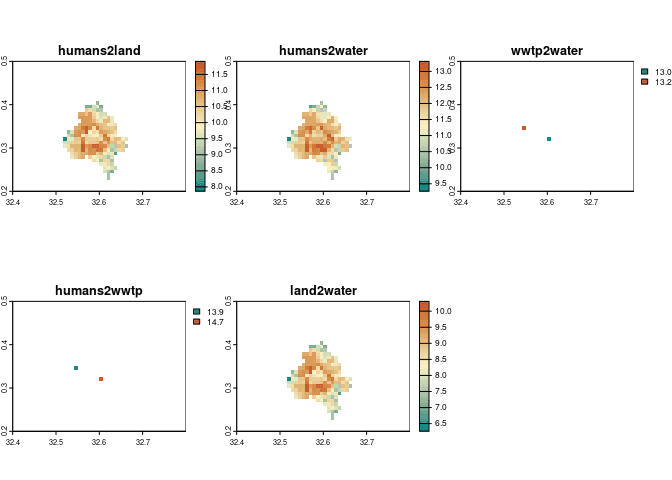
# read human emissions to surface water from the sanitation sources in each administrative area (tabular data)
df_humans_emissions <- read.csv(file.path(glowpa_run$settings$output$dir ,glowpa_run$settings$output$sources$human$surface_water))
# read gridded output
rast_surface_water <- terra::rast(file.path(glowpa_run$settings$output$dir, glowpa_run$settings$output$sinks$surface_water$grid))
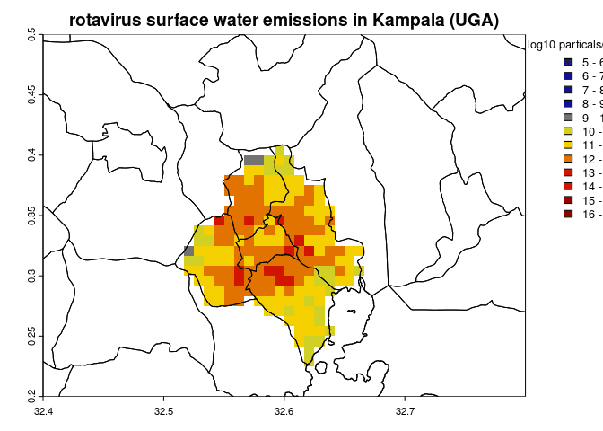
# download administrative boundaries of Uganda
uga = geodata::gadm('UGA',path = '.', level=3, resolution = 1)
# plot map of the log10 pathogen emissions per grid per year
terra::plot(log10(rast_surface_water), main='rotavirus surface water emissions in Kampala (UGA)', type='interval', breaks=seq(5,17), col= colorRampPalette(c("midnightblue","blue3","yellow","red3","darkred"), interpolate='linear')(12), plg=list(title='log10 particals/grid/year'))
# plot boundaries
terra::plot(uga,add=T)
6 Contributing
6.1 Setup Development Environment
You can use RStudio or Docker to setup a development environment. A Docker image including RStudio and project dependencies are available inside the git project.
RStudio
Step 1: Get the source code
git clone https://git.wur.nl/glowpa/glowpa-r.git
Step 2: Install dependencies:
# somehow renv does not resolve the git repo when using install and fails to find the package on the CRAN repo.
renv::install(exclude = "pathogenflows")
renv::install("git::https://git.wur.nl/glowpa/pathogenflows.git@be452603dc14512b57c3288635bec0960f7d9ce4")
RStudio Docker
Step 1: Install Docker and Docker Compose
Step 2: Get the source code
git clone https://git.wur.nl/glowpa/glowpa-r.git
Step 3: Run
cd glowpa
docker compose build rstudio
docker compose up rstudio -d
It will take a while before the Docker Image is built, because it will install all depending project dependencies. Rstudio Server runs on port 8989 and the glowpa folder is a shared volume on your host machine. Nagivate to localhost:8989.
Step 4:
Open the glowpa RStudio project.
6.2 Contribution Workflow
Step 1: Follow instructions in Setup Development Environment.
Step 2: Create an GitLab issue and describe the changes you want to implement in the model.
Step 3: Create a new feature branch from the GitLab issue.
Step 4: Fetch the newly created feature branch from the remote
repository and checkout the feature branch. The feature-branch can be
any name generated from the GitLab issue.
git fetch
git checkout feature-branch
Step 5: Implement, commit and push new changes to the feature branch. Please following our (code) conventions.
Step 6: Create a GitLab merge request to start the review process.
Step 7: Once the reviewer accept your changes your changes will be merged with the main model source code.
6.3 Contributing Conventions
-
Run tests and perform an automatic check if the package can be build and installed. Fix all failed tests and warnings.
devtools::check(error_on = "warning") -
Use the
stylerandlintrpackages to style the code files in theRdirectory to improve code readability.# automatic styler styler::style_dir("R") # try to solve most of the found warning from the lintr lintr::lint_dir("R") -
Document (exported) functions and data using
roxygenand generate automatic documentation.devtools::document() -
Bump the version number once the code is ready to be merged to the main branch. We follow the tidyverse package version conventions for our stable and in-development versions.
<major>.<minor>.<patch>        # released version
<major>.<minor>.<patch>.<dev>  # in-development version
usethis::use_version() -
Please keep the model documentation in the README file up to date.
6.4 Test Suite
Unit and regression tests are made using the testthat package. An
overall test-report is
available. The regression tests currently generates
maps and reports from
the land and surface water pathogen emissions which can are compared
against earlier versions. Moreover, snapshot tests are included to
detect any changes in model output values by running three model setups.
Kampala Model
Uganda Livestock Model
Rhine basin Model
6.5 Manage Packages
Check status of development environment.
renv::status(dev = T)
Updating the package lock file for development.
renv::snapshot(type = "explicit", dev = T)
Datasets
The GloWPa model installation includes a global dataset at 0.5 degree resolution which can be used as an example. The used input datasets are described in the sections below.
Global Gridded Population
Data source used to create global gridded population data.
Source: WorldPop - Population Counts - Unconstrained global mosaics
2000-2020 (1km)
Citation(s): WorldPop (2018)
Global Population Dynamics
The fraction urban population at country level has been taken from the world urbanization prospects 2018.
Source: United Nations, Department of Economic and Social Affairs,
Population Division (2018). World Urbanization Prospects: The 2018
Revision.
Citation(s): United Nations, Department of Economic and Social Affairs,
Population Division (2018)
The fraction of young children at country level has been taken from the world population prospects 2019
Source: United Nations, Department of Economic and Social Affairs,
Population Division (2019). World Population Prospects 2019, Online
Edition. Rev. 1
Citation(s): United Nations, Department of Economic and Social Affairs,
Population Division (2019)
Human Development Index (HDI)
Source: United Nations Development Programme - Human Development
Index
Citation(s): Programme United Nations Development (2024)
Pathogen Properties
Incidence, shedding rate and shedding duration are based on literature and explained in Hofstra et al. (2013) for cryptosporidium and Kiulia et al. (2015) for rotavirus.
The data used to estimate the decay of cryptosporiudium in livestock manure storage can be found in Vermeulen et al. (2017). Properties used to calculate the decay during transport from land to water and inside rivers are described by Vermeulen et al. (2019).
Sanitation
The fraction of population with access to various levels of sanitation at country level are taken from the WHO/UNICEF JMP global database. The JPM sanitation classification has been re-classified to flushSewer(1), flushSeptic(2), flushPit(3), flushUnknown(4), flushOpen(5), pitSlab(6), pitNoSlab(7), hangingToilet(8), bucketLatrine(9), compostingToilet(10), openDefecation(11) and other(12).
Source: https://washdata.org/data/downloads
citation(s): World Health Organization and UNICEF (2023)
Waste Water Treatment
Based on the model configuration either grid or point level treatment is applied.
grid level treatment
The treatment data has been taken from the work of Puijenbroek et al.
(2019) at country level. The values can be
found in the supplementary
data
of the paper.
The removal and liquid fractions are taken from the sketcher tool of Matt Verbyla. Ultimately, fEmitted_inEffluent_after_treatment is used in the GloWPa model, not any of the other variables from this part.
point level treatment
The HydroWASTE v1.0 dataset has been used to select the location of
waste water treatment plants. The WWTP’s are only considered when the
status is either ‘not reported’ (assumed operational) or operational.
The emitted fraction is estimated based on the treatment level and
pathogen type.
Source: HydroWASTE v1.0
Citation: Ehalt Macedo et al. (2022)
Hydrology
surface runoff and river discharge
The VIC model is used to produce daily surface runoff and river
discharge based on WATCH forcing data. The model output is averaged over
the period 1970-2000 to produce 30-year monthly climatology (Vermeulen
et al., 2019).
flow direction
The 0.5 degrees flow direction is based in the global flow direction map
DDM30 (Döll & Lehner, 2002) which is also used to
produce the river discharge using the VIC model.
river geometry and residence time
The river geometry equations are taken from Leopold & Maddock
(1953) to calculate river width, depth and flow
velocity from river discharge. More details can be found in Vermeulen et
al. (2019).
water temperature
The monthly mean river water temperature are taken from estimates by the
VIC-RBM model framework (Vliet et al., 2012).
DOC
The Global Nutrient Export from Watersheds (Global NEWS) model provides
estimates of river export of DOC for the world (Harrison et al.,
2005; Mayorga et al., 2010).
Meteorology
solar radiation and air temperature
Monthly climatology is created from the WATCH forcing data over the
period 1970-2000 (Weedon et al., 2011).
Livestock
animal heads
*Species: cattle, sheep, goats, pigs, chickens, and ducks *
Source: GLW - Gridded Livestock of the World (~1km)
Citation: Robinson et al. (2014)
Species: buffaloes, horses, camels, mules, and donkeys
Source: FAOSTAT (heads) and GLW (spatial distribution)
Citation: Food and Agriculture Organization of the United Nations (FAO)
(2024) and Robinson et al.
(2014)
body mass
Source: IPCC guidelines for National Greenhouse Gas inventories
Citation: IPCC (2006)
excretion rates and prevalence
Literature
Review
manure production Source: IPCC guidelines for National
Greenhouse Gas inventories
Level: continent level Citation(s): IPCC (2006)
intensive and extensive farming systems
Source: IMAGE model based on FAO report
Citation(s): Bouwman et al. (2013)
manure storage systems
cattle, buffaloes, pigs
Source: IPCC Guidelines for National Greenhouse Gas Inventories
(2006)
level: continent level
Citation: IPCC (2006)
chickens, ducks, sheep, goats, buffaloes, horses, asses, camels
Source: USEPA report on Global methane emissions from livestock and
poultry manure
level: country level
Citation: Safley et al. (1992)
References
Bouwman, L., Goldewijk, K. K., Van Der Hoek, K. W., Beusen, A. H. W., Van Vuuren, D. P., Willems, J., Rufino, M. C., & Stehfest, E. (2013). Exploring global changes in nitrogen and phosphorus cycles in agriculture induced by livestock production over the 1900-2050 period [Journal Article]. Proceedings of the National Academy of Sciences of the United States of America, 110(52), 20882–20887. https://doi.org/10.1073/pnas.1012878108
Döll, P., & Lehner, B. (2002). Validation of a new global 30-min drainage direction map [Journal Article]. Journal of Hydrology, 258(1), 214–231. https://doi.org/https://doi.org/10.1016/S0022-1694(01)00565-0
Ehalt Macedo, H., Lehner, B., Nicell, J., Grill, G., Li, J., Limtong, A., & Shakya, R. (2022). Distribution and characteristics of wastewater treatment plants within the global river network [Journal Article]. Earth Syst. Sci. Data, 14(2), 559–577. https://doi.org/10.5194/essd-14-559-2022
Food and Agriculture Organization of the United Nations (FAO). (2024). FAOSTAT (Vol. 2024) [Dataset]. https://www.fao.org/faostat/en/#data/QCL
Harrison, J. A., Caraco, N., & Seitzinger, S. P. (2005). Global patterns and sources of dissolved organic matter export to the coastal zone: Results from a spatially explicit, global model [Journal Article]. Global Biogeochemical Cycles, 19(4). https://doi.org/https://doi.org/10.1029/2005GB002480
Hofstra, N., Bouwman, A. F., Beusen, A. H., & Medema, G. J. (2013). Exploring global cryptosporidium emissions to surface water [Journal Article]. Sci Total Environ, 442, 10–19. https://doi.org/10.1016/j.scitotenv.2012.10.013
Hofstra, N., & Vermeulen, L. (2016). Impacts of population growth, urbanisation and sanitation changes on global human cryptosporidium emissions to surface water [Journal Article]. International Journal of Hygiene and Environmental Health, 219. https://doi.org/10.1016/j.ijheh.2016.06.005
IPCC. (2006). 2006 IPCC guidelines for national greenhouse gas inventories (Vol. 4) [Report]. Institute for Global Environmental Strategies.
Kiulia, N. M., Hofstra, N., Vermeulen, L. C., Obara, M. A., Medema, G., & Rose, J. B. (2015). Global occurrence and emission of rotaviruses to surface waters [Journal Article]. Pathogens, 4(2), 229–255. https://www.mdpi.com/2076-0817/4/2/229
Leopold, L. B., & Maddock, T. (1953). The hydraulic geometry of stream channels and some physiographic implications (Vol. 252) [Book]. US Government Printing Office.
Mayorga, E., Seitzinger, S. P., Harrison, J. A., Dumont, E., Beusen, A. H. W., Bouwman, A. F., Fekete, B. M., Kroeze, C., & Van Drecht, G. (2010). Global nutrient export from WaterSheds 2 (NEWS 2): Model development and implementation [Journal Article]. Environmental Modelling & Software, 25(7), 837–853. https://doi.org/https://doi.org/10.1016/j.envsoft.2010.01.007
Programme United Nations Development. (2024). Human development index [Dataset]. https://hdr.undp.org/sites/default/files/2023-24_HDR/HDR23-24_Statistical_Annex_HDI_Table.xlsx
Puijenbroek, P. J. T. M. van, Beusen, A. H. W., & Bouwman, A. F. (2019). Global nitrogen and phosphorus in urban waste water based on the shared socio-economic pathways [Journal Article]. Journal of Environmental Management, 231, 446–456. https://doi.org/https://doi.org/10.1016/j.jenvman.2018.10.048
Robinson, T. P., Wint, G. R. W., Conchedda, G., Van Boeckel, T. P., Ercoli, V., Palamara, E., Cinardi, G., D’Aietti, L., Hay, S. I., & Gilbert, M. (2014). Mapping the global distribution of livestock [Journal Article]. PLOS ONE, 9(5), e96084. https://doi.org/10.1371/journal.pone.0096084
Safley, L. M., Casada, M. E., Woodbury, J. W., & Roos, K. F. (1992). Global methane emissions from livestock and poultry manure [Report]. United States Environmental Protection Agency (USEPA).
United Nations, Department of Economic and Social Affairs, Population Division. (2018). World urbanization prospects: The 2018 revision, online edition [Dataset]. United Nations. https://population.un.org/wup/Download/
United Nations, Department of Economic and Social Affairs, Population Division. (2019). World population prospects 2019, online edition. Rev. 1 [Dataset]. United Nations. https://population.un.org/wpp2019/Download/Standard/Population/
Vermeulen, L. C., Benders, J., Medema, G., & Hofstra, N. (2017). Global cryptosporidium loads from livestock manure [Journal Article]. Environmental Science & Technology, 51(15), 8663–8671. https://doi.org/10.1021/acs.est.7b00452
Vermeulen, L. C., van Hengel, M., Kroeze, C., Medema, G., Spanier, J. E., van Vliet, M. T. H., & Hofstra, N. (2019). Cryptosporidium concentrations in rivers worldwide. Water Research, 149, 202–214. https://doi.org/https://doi.org/10.1016/j.watres.2018.10.069
Vliet, M. T. H. van, Yearsley, J. R., Franssen, W. H. P., Ludwig, F., Haddeland, I., Lettenmaier, D. P., & Kabat, P. (2012). Coupled daily streamflow and water temperature modelling in large river basins [Journal Article]. Hydrol. Earth Syst. Sci., 16(11), 4303–4321. https://doi.org/10.5194/hess-16-4303-2012
Weedon, G. P., Gomes, S., Viterbo, P., Shuttleworth, W. J., Blyth, E., Österle, H., Adam, J. C., Bellouin, N., Boucher, O., & Best, M. (2011). Creation of the WATCH forcing data and its use to assess global and regional reference crop evaporation over land during the twentieth century [Journal Article]. Journal of Hydrometeorology, 12(5), 823–848. https://doi.org/https://doi.org/10.1175/2011JHM1369.1
World Health Organization and UNICEF. (2023). Estimates for drinking water, sanitation and hygiene services by country (2000-2022) [Dataset]. https://washdata.org/data/downloads
WorldPop. (2018). Global high resolution population denominators project [Dataset]. School of Geography; Environmental Science, University of Southampton; Department of Geography; Geosciences, University of Louisville; Departement de Geographie, Universite de Namur; Center for International Earth Science Information Network (CIESIN), Columbia University; University of Southampton. https://doi.org/10.5258/SOTON/WP00647


